Case Studies

To demonstrate the methods and tools developed under FASTWATER, two case study regions were modelled using mesh refinement:

1. The EMEC Tidal Energy Site, Falls of Warness, Orkney Islands

2. The Inner Sound, Pentland Firth

The EMEC site has been chosen as there is a large volume of legacy data collected for this site, the information about this site is in the public domain so the results can be be provided as open data, and there is on-going work with Orbital who have recently deployed their O2 floating twin-trubine device in the northwest of the EMEC site.

The Inner Sound is where the Simec-Atlantis MeyGen tidal turbine array is situate. The model developed in for this region provides Simec-Atlantis detailed information about the 3-D hydrodynamics and its potential impact on turbine perfomance, and will aid the decision making related to future device siting for array expansion.

EMEC Tidal Energy Test Site, Falls of Warness, Orkney Islands

There are two end-use targets for the models of the EMEC tidal energy site:

1. Determine whether the observed significant differences in tidal flow strcuture from a pair of ADCP’s deploy either side of the DeepGen IV TEC (approximately 80m appart) during the ReDAPT project can be explained by the regional dynamics.

2. Generate a base set of fluid velocity data for input to a one-way coupled wave model of the EMEC site. The wave model predictions will be used to provide an estimate of of wave direction information for site wave data based on pressure sensor measurements of surface elevation.

The first use case requires a model that resolves the dominant 3-D flow structures in and around the deployment site, while the second use case can be based on a low-resolution model in the first instance. For the second case the FASTWATER base model ouput will suffices, the specifciation and design are describe in Base Model. The model design specification for Use Case 1 will be described here.

FoW Model Design Specification

The model design aims to investigate possible reasons for the observed differences in flow structure between a pair of in situ measurement sites (TD7_01, TD7_02; see Figure 1), separated by approximately 80m, in the Falls of Warness, Orkneys. These data were collected during the ReDAPT project, while the Alstrom DeepGen IV tidal turbine was installed and operating. The turbine was mid-way between the two instruments. The placement of the instruments meets an IEC specification for power assessment, and are not directly affected by the turbine wake on either phase (flood or ebb) of the tide.

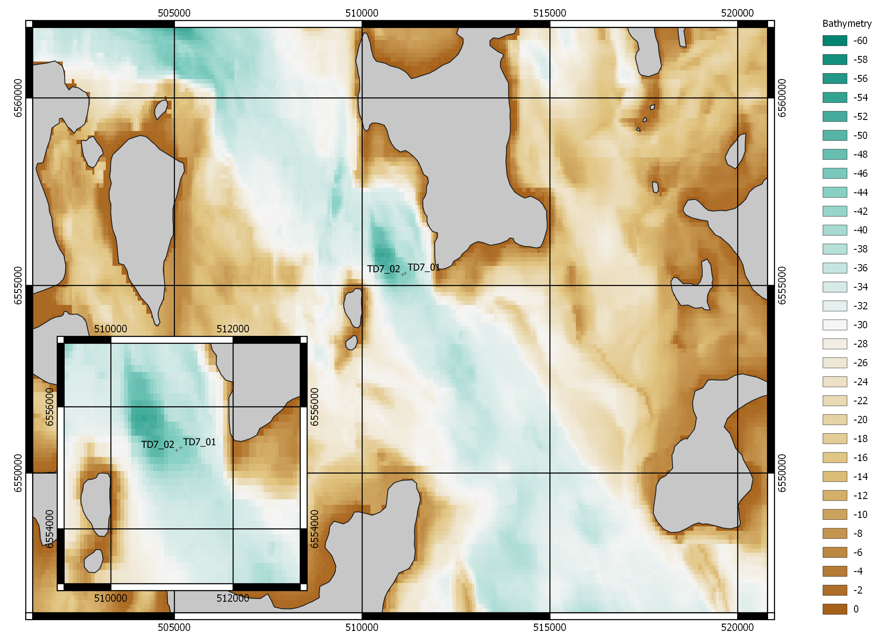
Figure 1. Falls of Warness site map. TD7_01 and TD7_02 are the locations of the in situ measurements. The inset shows the proximity of TD7_01 to a natural shelf in the bathymetry.

The hypothesis is that the formation a strong shear layer on the northern side of the channel will impact the flow structures at the TD7_01 location more than at the TD7_02 location. The formation of this shear layer may vary between flood (flow from the west) and ebb (flow from the east) tides. To resolve the shear layers the mesh resolution must be high enough to resolve eddy scales at least comparable to the water depth. The location of this shear layer may be affected by headland eddy sheading and by trapped eddies forming in the bay on the north side of the channel.

Two separate mesh designs are consider to better understand the impact of the fluid dynamics:

1. Mesh growth rate based on distance from the nearest coast.

2. Mesh growth from regions of high vorticity.

The refinement region is limited to the Falls of Warness region, to keep the total number of mesh nodes within the 100k limit to minimise computational cost and data volumes.

The minimum mesh resolution targetted is 30m, maximum outer domain resolution 10km, 15 sigma layers will be used to capture the vertical flow structures, and the timestep needs to ensure a reasonable level of solution convergence.

The bathymetric data should of a comparable resolution to that of the mesh.

Tidal forcing of the open boundary of the model domain should include as many harmonic as available from an appropriate tidal atlas.

The OpenTelemac open-source software will be used to solve the 3-D hydrodynamic equations of motion.

FoW Mesh Construction

The BlueKenue software tools developed by the National Research Council of Canada were used to generate the model meshes. This tool has been developed for use with the OpenTelemac tools and creates the required proprietary files formats used by OpenTelemac. The BlueKenue tools can load ESRI shapefiles used to define coastlines, domain boundaries, internal hard lines and points, etc. It also can load information in various ASCII formats. The majority of the contraining data were generated using the QGIS open-source Geospatial Information System software.

The BlueKenue tool provides two methods for building a mesh:

1. A fixed growth rate from the hard boundary lines.

2. A mesh density defined across the mesh domain.

Both methods respect the underlying resolution along the boundary lines, then grow the mesh as efficiently as possible based on the method used. The final outer boundary target resolution is provided the set the mesh resolution limits require.

The meshes were constructed using a two-stage process:

1. An inner mesh was constructed over the Falls of Warness using one of the two refinement methods.

2. The full domain mesh was constructed around this inner sub-mesh using a constant growth rate out to a edge length of 10km.

The starting point for the coastline data is the 250m resolution coastlines used to construct the FASTWATER base model, and the same growth rate was used to generate the final full domain mesh from the sub-mesh, this helps maintain a minimum nuber of the model nodes, and keeps the far-field construct similar to that of the base model.

Distance-to-Coast (D2C) refinement

The mesh refinement region chosen is shown in Figure 2 below. The resolution of the coastline data was increased for all land boundaries within this domain, with a suitable gradual increase to the nominal 250m resolution of the base model data outside the sub-domain, to ensure a reasonable growth of the mesh outwith the sub-mesh.

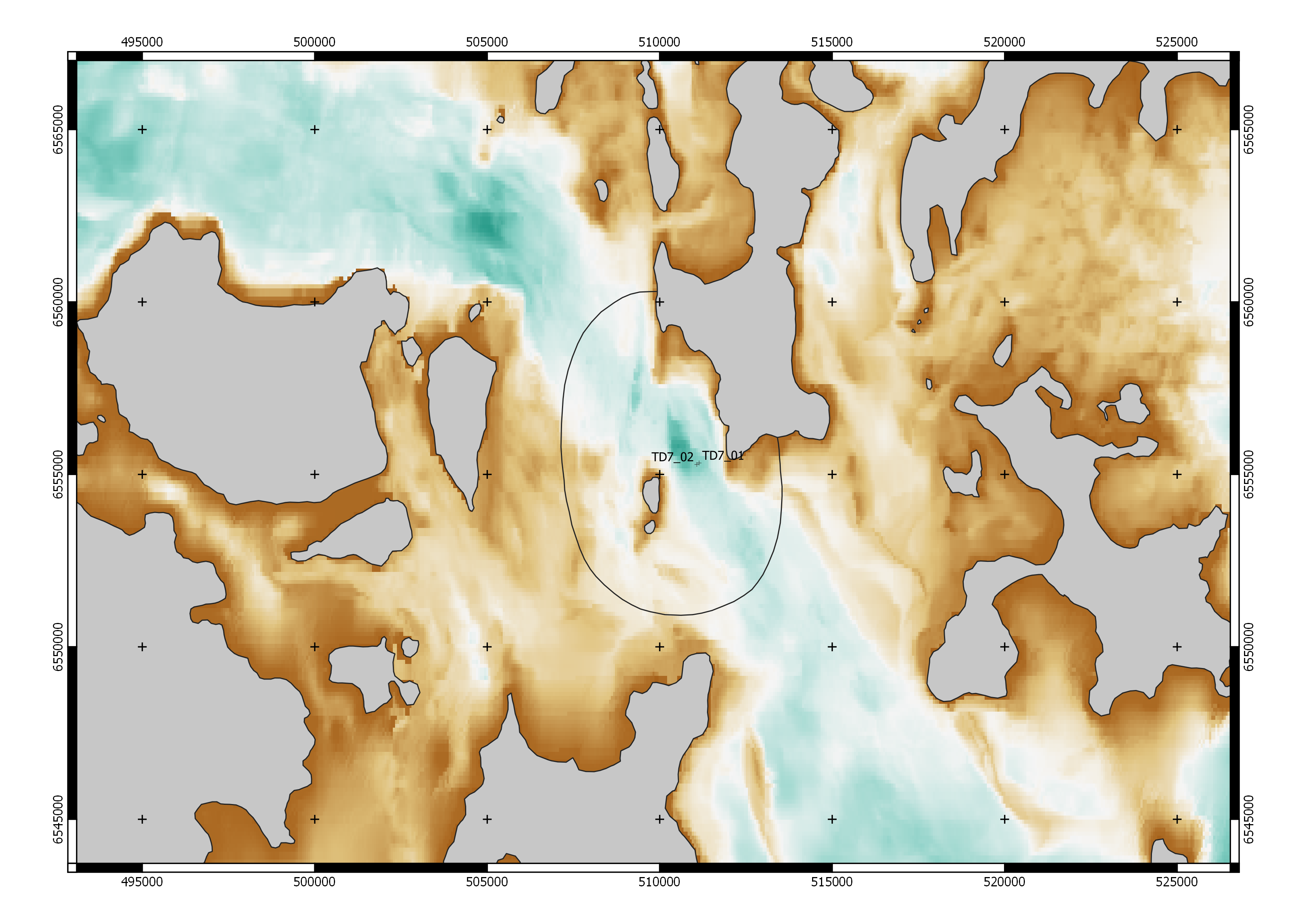
Figure 2. Falls of Warness refinement region used to build the sub-mesh. The area aims to capture flow separation at the headland, the influence of the smaller islands in the channel, and the trapped eddy foramtion area.

The distance-to-coast refinement used a density map generated from the coastline shapefiles and the nodes from a high-resolution model mesh generated for the full domain, creating a map of D2C across the model domain. The distance-to-coast was generated using the otmCoastalDistance.py processing script that is available in the /scripts/telemacModelData directory of the FASTWATER GitLab repository. This was then converted into a mesh density based on the sub-mesh domain extent, where the density value corresponds the target element edge-length for the node location. The function used to convert D2C to an edge length is:

\(\rho_i = ( [ l_{max} - l_{min} ] / d_{max} ) d_i + l_{min}\)

where :math:’l_{min}` was set to 30m, :math:’l_{max}` was set to 100m, and :math:’d_{max}` was set to 1000m. The conversion was done within BlueKenue using the built-in Calculator tool. The resulting file was then passed to the mesh generator as the density function. The resutling mesh is shown in Figure 3.

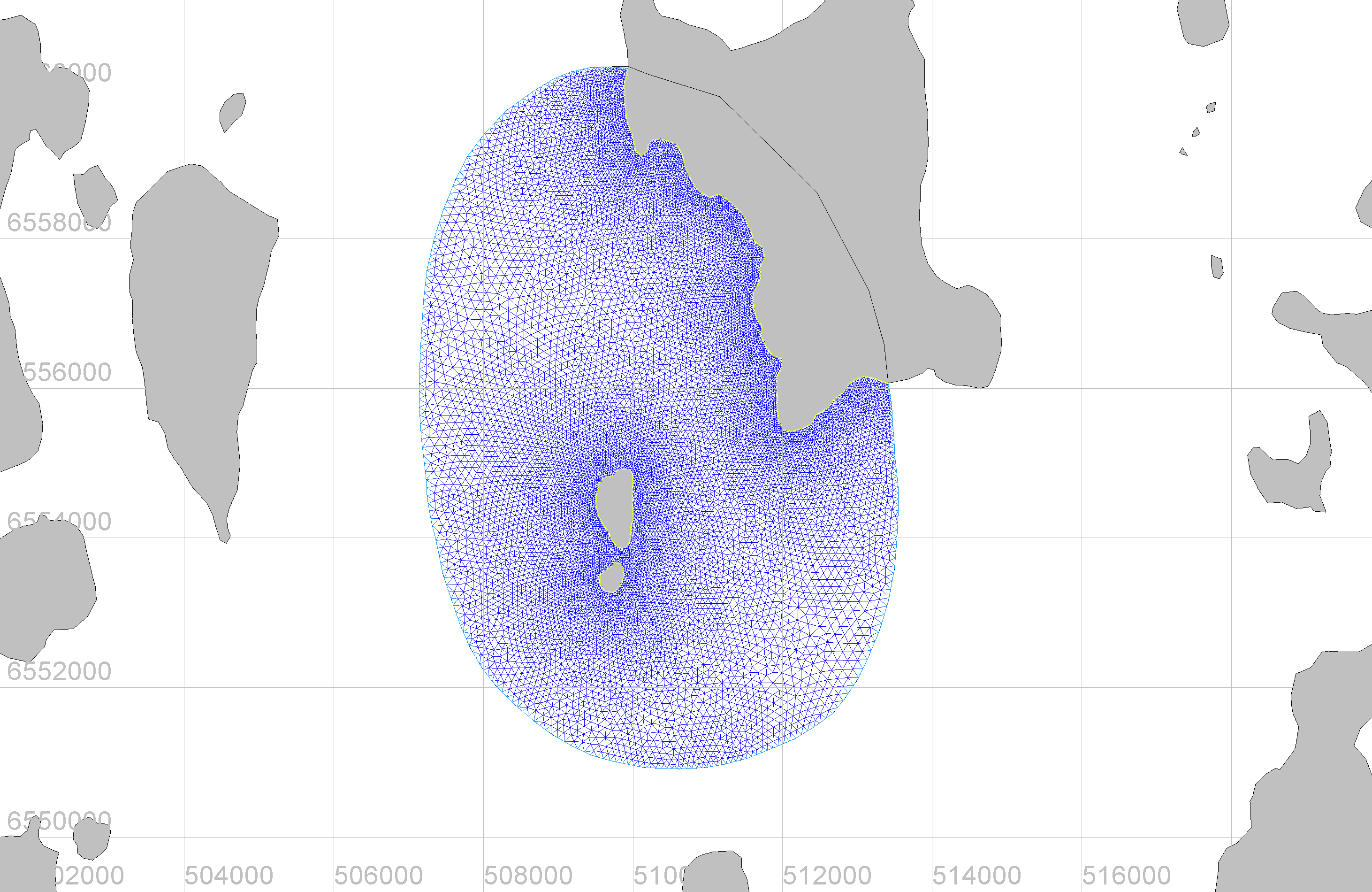
Figure 3. Falls of Warness refinement sub-mesh generated in BlueKenue using the distance-to-coast density data.

Table 1: Falls of Warness D2C sub-mesh characteristics

Mesh Parameter	Value
Number of Nodes	12205
Number of Edge Nodes	685
Minimum Edge Length	21.0m
Maximum Edge Length	137.6m
Mean Edge Length	45.9m

Vorticity-base (VORT) refinement

The 2-D vorticity field generated from the depth-avearaged velocity output of the D2C refinement model was used to create a spatial map of square root of the maximum absolute vorticitiy across the full model domain. The square root was used to non-linearly spread the data to simplify the identification of areas of maximum vorticity. From this map a set of hard lines identifying the core regions of maximum vorticity were created in QGIS and converted in to an ESRI shapefile that was passed to BlueKenue to define a set of hardlines used to grow the mesh from. The resolution of points along the vorticity-based hardlines was set to 30m for highest vorticity growing to approximately 100m for the lowest levels of vorticity along the lines.

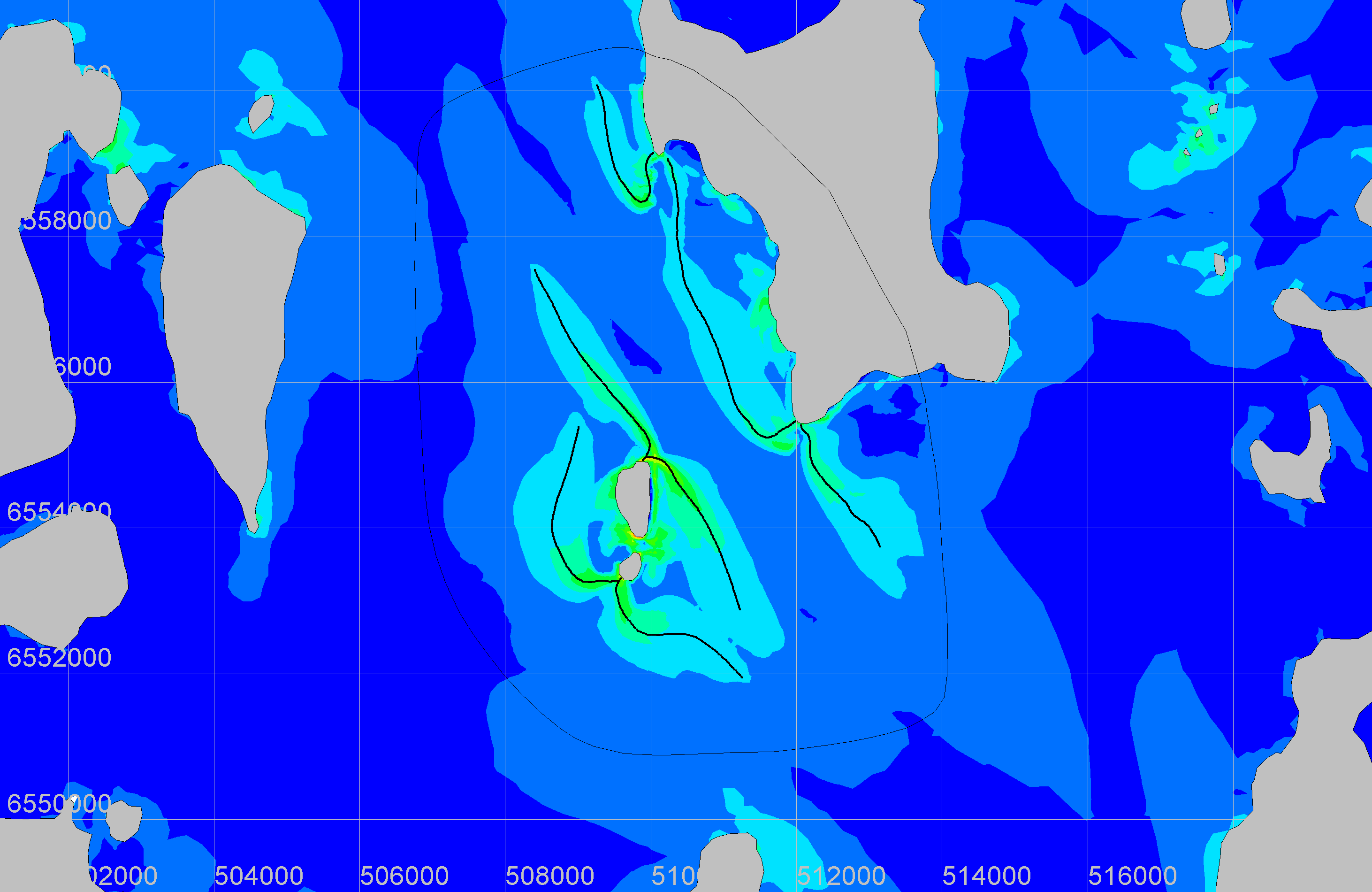
Figure 4. Map of the maximum vorticity for the Falls of Warness based on the 2-D depth-averaged velocity data generated by the D2C refinement model.

Based on the location of these regions of vorticity, the sub-mesh domain extent was redefined so that the core of the high vorticity regions did not cross the sub-mesh boundary, this new domain extent is shown in Figure 5.

Figure 5. Falls of Warness refinement region used to build the vorticity-based sub-mesh. The area aims to capture all of the core areas of maximum vorticity as identified by the D2C model velocity data.

A growth rate of 1.05 and a maximum target edge length of 150m was used to build the mesh. The 250m coastline data had to be refined down to 30m resolution within the sub-mesh domain, with an appropriate gradual increase back to the nominal 250m resolution away from the sub-domain. The resulting sub-mesh is shown in Figure 6.

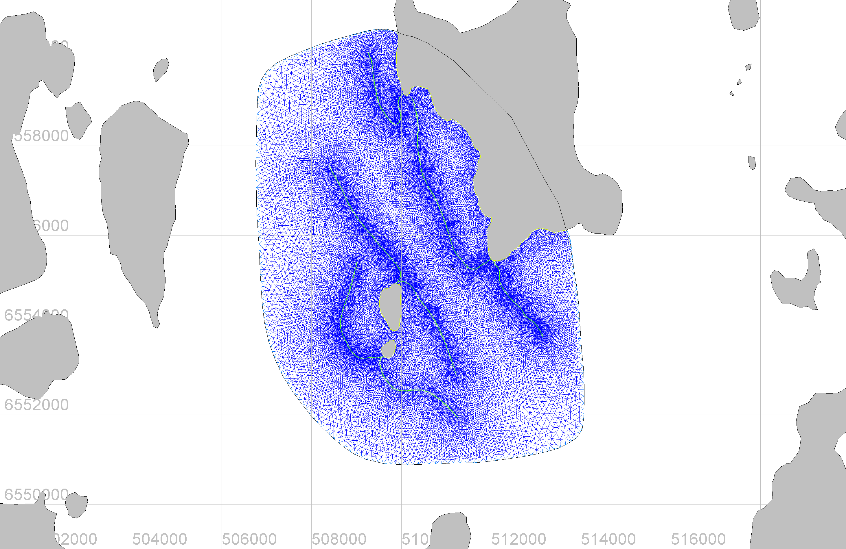
Figure 6. Falls of Warness vorticity-based refinement sub-mesh generated in BlueKenue using the 2-D depth average vorticity data generated from the D2C model output.

The key mesh parameters are summarised in the following table:

Table 2: Falls of Warness VORT sub-mesh characteristics

Mesh Parameter	Value
Number of Nodes	39281
Number of Edge Nodes	647
Minimum Edge Length	7.8m
Maximum Edge Length	220.4m
Mean Edge Length	34.5m

Full-Domain mesh

The full mesh was generated around the sub-mesh using the 250m resolution coastline data with a growth rate of 1.2 (shown in Figure 7)and a maximum outer domain target edge length of 10km. The resulting key mesh parameters for the D2C and VORT full meshes are summarised in the table below.

Table 3: Falls of Warness full domain mesh characteristics for the D2C and VORT models

Mesh Parameter	D2C	VORT
Number of Nodes	54629	81733
Number of Edge Nodes	8758	8846
Minimum Edge Length	21.1m	7.8m
Maximum Edge Length	9999.8m	14735.0m
Mean Edge Length	216.7	267.7m

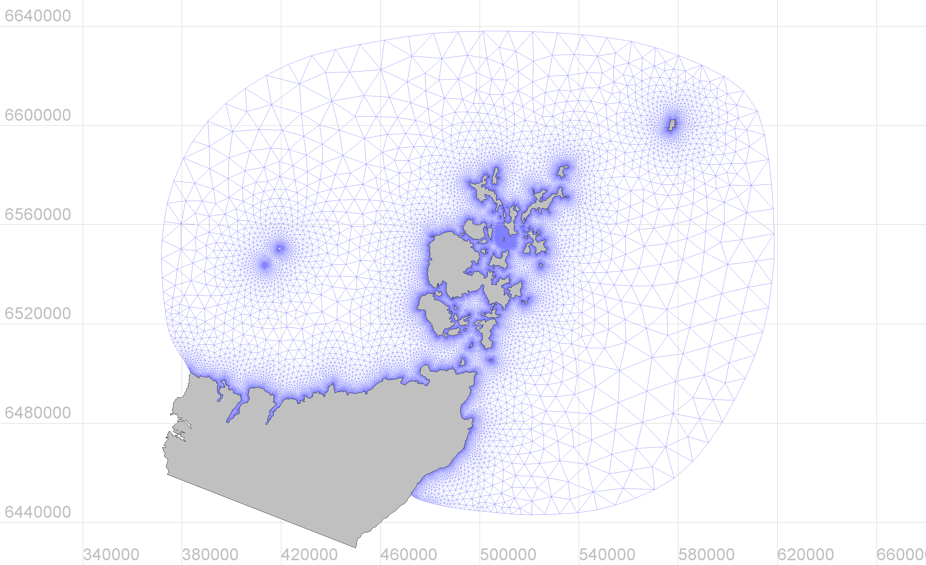
Figure 7. The full domain mesh including the Falls of Warness vorticity-based refinement region.

FoW Boundary Conditions

The model vertical constraint is defined by the bathymetric depth across the model domain. The EMODNet astronomic mean low tide bathymetry + topography data were used as the basis for the bathymetry, these were then nominally corrected to mean sea level (MSL) using the spring tide range data available from the Renewables Atlas. It is possible to get MSL correct data from the EMODNet archive, but is was found that the correction next to the coast was out by up to 7m, hence the reason for using the AMLT data with a manual correction to MSL. These data are interpolated onto the mesh using the interpolation tool in Bluekenue.

A spatially varying map of the friction coefficient was used to define the bottom boundary friction. This map was generated using the EMODNet seabed habitats data which provides shapefiles of polygons with a substrate type classification string. Using QGIS, these classes were mapped to C₁₀₀ drag coefficients taken from the literature, and the resulting data then mapped onto the EMODNet bathymetry locations and saved as a shapefile. A range of bottom friction coefficient values were then calculated from the C₁₀₀ values and saved in the shapefile. These data can be loaded into BlueKenue and interpolated onto any mesh using the built-in interpolation tool.

Open boundary forcing was based on the OSU TPXO tidal atlas 1/30 degree data for the European Shelf. These data are readily integrated with the OpenTelemac solver and give a sufficient number of tidal constituents to force the model.

FoW Numerical Scheme

The model is run in 3D mode using the non-hydrostatic setting.

Coriolis forcing is turned on, with the coefficient set to \(1.25 \times 10^{-4}\) (this corresponds approximately to the value at the Falls of Warness).

Tidal boundary forcing is via the tidal harmonics provided by the OSU TOPEX European Shelf (2008) tidal atlas data. The minor constituent interference is included in the computation of the tidal forcing.

Liquid boundary conditions solved using the Thompson method based on characteristics.

Wetting/Drying is turned on with the N-S equations solved everywhere with a free-surface gradient correction on tidal flats. Negative depths a corrected using a flux control method. To optimise computation time, void volumes are skipped.

Horizontal turbulence is modelled using the Smagorinsky scheme (recommended in the OpenTelemac Users Guide).

Vertical turbulence is modelled using a Prandtl mixing length parematerisation, with a coefficient for the vertical diffusion of velocity set to \(1.0 \times 10^{-6}\), and the Munk and Anderson damping function applied. The turbulence regime for the solid boundaries is set to rough.

Preconditioning for the propagation steps and Poisson Pressure Equation are set to diagnonal and direct solver on the vertical respectively.

FoW Model Validation

The model has been validated against the in situ ADCP data collected during the ReDAPT project at the TD7_01 and TD7_02 locations. The first step in the process is to extract timeseries of the velocity profiles from the 3-D model output at these two locations. The script extract_by_location.py provided in the /scripts/telemacModelData directory of the FASTWATER repository, is used for this purpose. The coniguration files fow_d2c_redapt_adcp_locations_utmz30.txt and fow_vort_redapt_adcp_locations_utmz30.txt define where to extract the data from and what time periods to cover. These timeseries are then preprocessed to generate data at specified heights above the bed. It is know from the in situ measurements that there is a complex structure to the vertical velocity shear profile which varys with time. The script used to apply the preprocessing is preprocess_fow.py provided in the /scripts/modelValidation directory of the FASTWATER repository.

To investigate the vertical variation in flow strucutre, three levels corresponding to three differenct turbine design hub heights were chosen for the analysis. The turbines replicated are (1) Sabella D10, (2) Alstrom DeepGenIV (the turbine associated with the ReDAPT project), and (3) the Orbital Marine O2 floating turbine (currently install at the EMEC site). The relevant details for these turbines are given in the table below.

Table 4: Tidal turbine parameters used for data extraction and flow characterisation

Parameter	Sabell D10	Alstrom DeepGenIV	Orbial Marine 02
Rotor Diameter [ m ]	10	20	22
Hub Height [ m ]	11 (above bed)	18 (above bed)	14 (below surface)
Cut-In_Speed [ m/s ]	0.4	1.0	1.0
Rated Speed [ m/s ]	3.1	4.0	4.5
Moutning	Bottom	Bottom	Surface floating

The aim is to determine impact that a models ability to support a range scales associated coherent flow structures has on the model predictive skill, and to determine if the coherent flow structures are the only source of variability between the two locations. The preprocessed data from each of these heights was converted into flow characteristic diagrams, and these were compared with similar data collected from the base model at the TD7_01 and TD7_02 locations. The preprocessing scripts generate the relevant figures that characterise a site for a given vertical location in the water column.

Examples of the flow characterisation for the TEC_01 and TEC_02 locations based on the output from the FoW D2C model taken at the DeepGenIV hub height are shown below. Included in the figures are are the cut-in and rated speeds for the DeepGenIV turbine to give an indication of the potential impact of flow variation on the turbine perfomance.

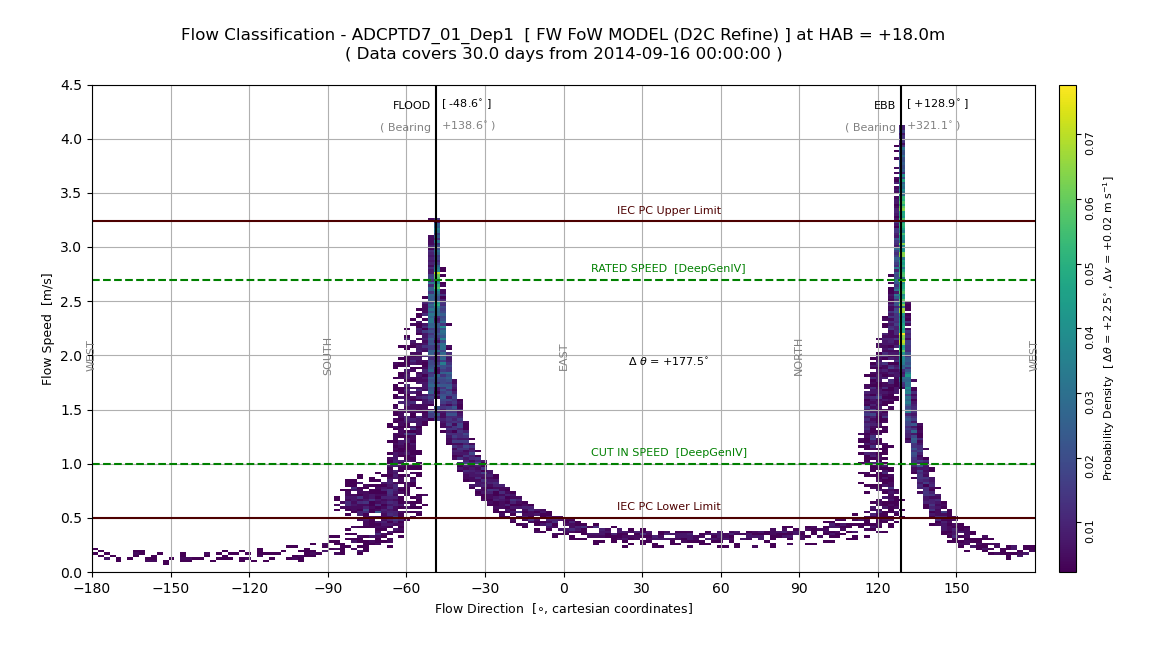
Figure 8. Falls of Warness D2C model flow characterisation at the TD7_01 measurement location for the DeepGenIV turbine hub height.

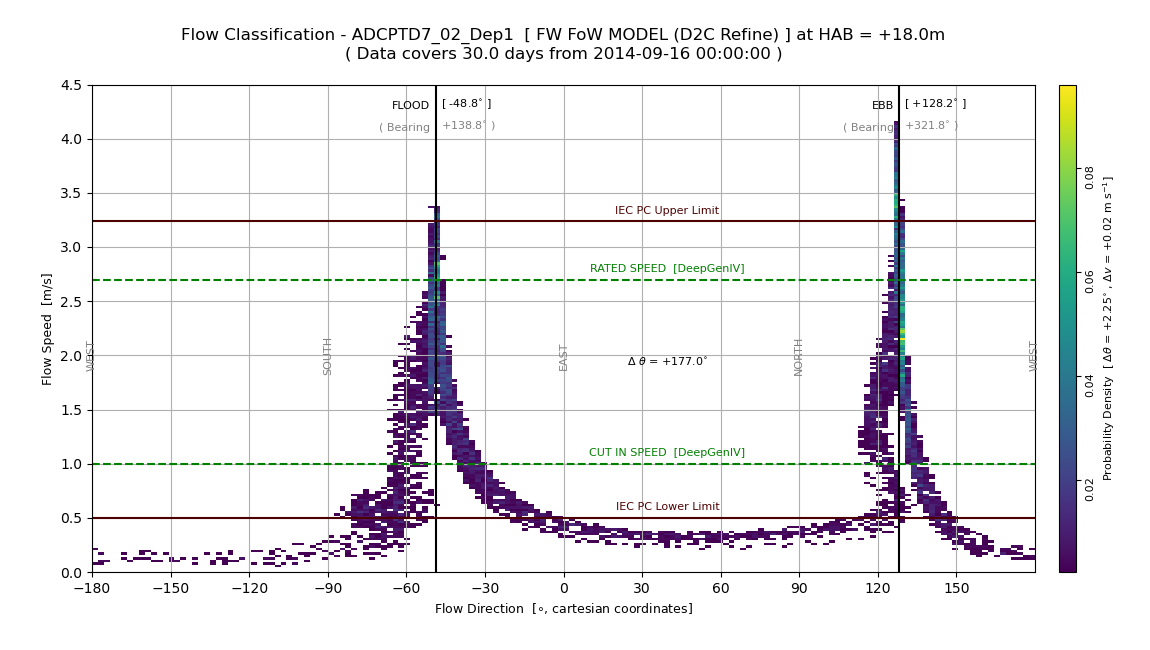
Figure 9. Falls of Warness D2C model flow characterisation at the TD7_02 measurement location for the DeepGenIV turbine hub height.

The same preprocessing was applied to the ReDAPT in situ measurements. The timeseries generated will be used to calculate model validation statistics based on the observations to determine how well the model is performing as a predictor of flow state. The flow characterisation figures for the two instruments at the DeepGenIV hub height are shown below. The script used to apply the preprocessing to the ReDAPT measurement data is preprocess_redapt.py provided in the /scripts/modelValidation directory of the FASTWATER repository. A 5-minute running mean was applied to the high-frequency instrument measurements to replicate the model output sampling. The data QC flags were used to remove low quality data prior to analysis.

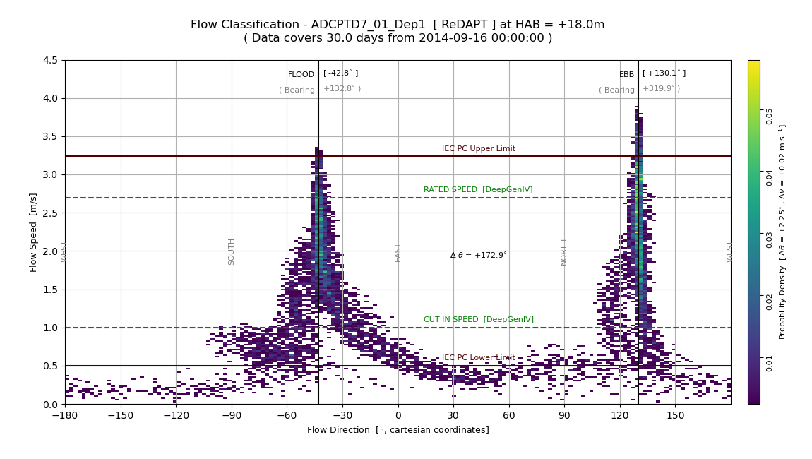
Figure 10. Falls of Warness D2C model flow characterisation at the TD7_01 measurement location for the DeepGenIV turbine hub height.

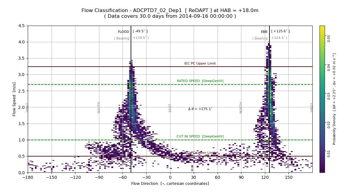
Figure 11. Falls of Warness D2C model flow characterisation at the TD7_02 measurement location for the DeepGenIV turbine hub height.

After the data preprocessing has been applied to both the model output and in situ measurements, the timeseries of model data are compared statistically to the observational data using the metrics provided in the :py:mod:`fastwater.general.statsTools`_ module and the validation processing functions supplied in the :py:mod:`fastwater.analysis.validation.py`_ module. The script validate_fow.py provided in the /scripts/modelValidation directory of the FASTWATER repository, was used to generate the validation statistics. The key outputs of the validation procees are summarised in the graphic generated by the :py:mod:`fastwater.analysis.validation.py`_ functions. The validation process is applied to the velocity magnitude and velocity directions separately. The summary graphics for the FoW D2C model velocity magnitudes at the two measurement sites for the DeepGenIV hub height are shown below.

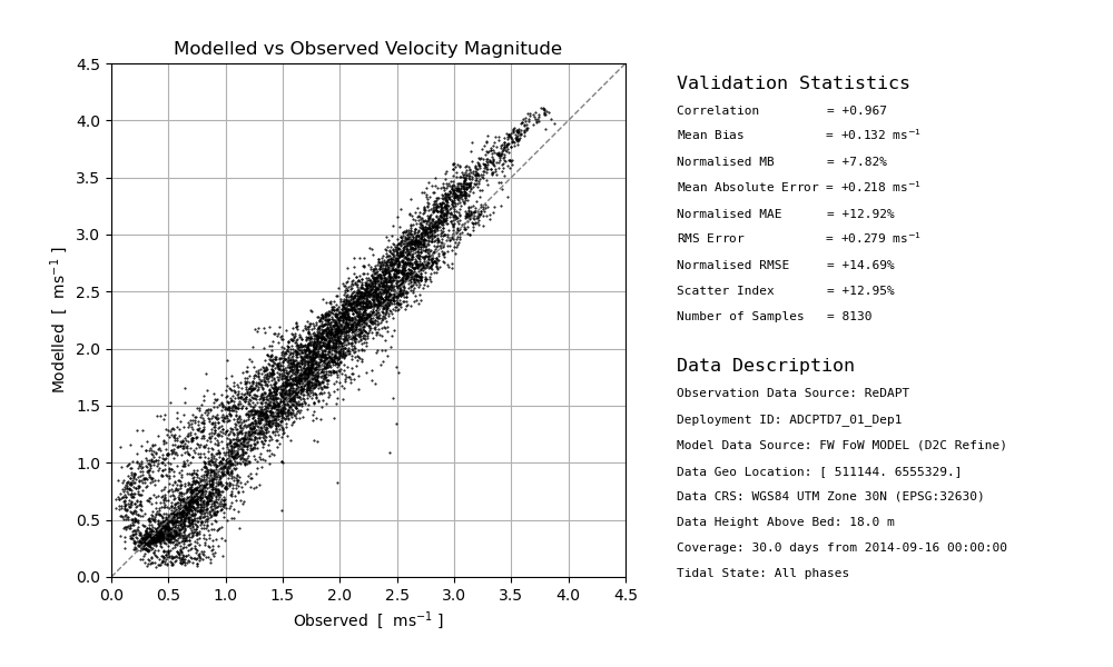
Figure 12. Validation of Falls of Warness D2C model velocity magnitude against the ReDAPT TD7_01 measurement for the DeepGenIV turbine hub height for the all tide states.

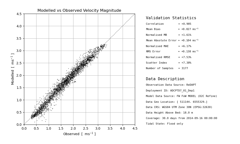
Figure 13. Validation of Falls of Warness D2C model velocity magnitude against the ReDAPT TD7_01 measurement for the DeepGenIV turbine hub height for flood tides.

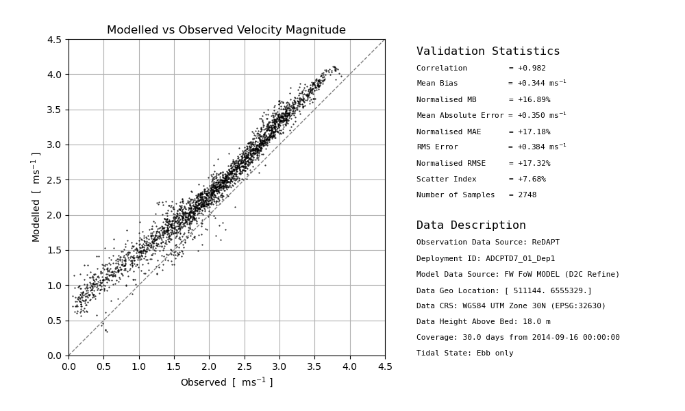
Figure 14. Validation of Falls of Warness D2C model velocity magnitude against the ReDAPT TD7_01 measurement for the DeepGenIV turbine hub height for ebb tides.

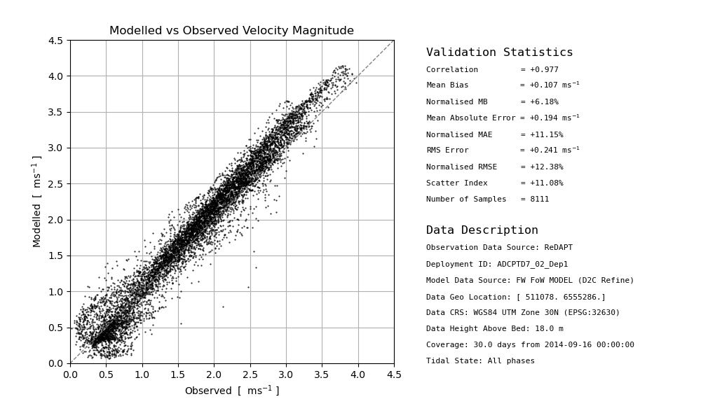
Figure 15. Validation of Falls of Warness D2C model velocity magnitude against the ReDAPT TD7_02 measurement for the DeepGenIV turbine hub height for the all tide states.

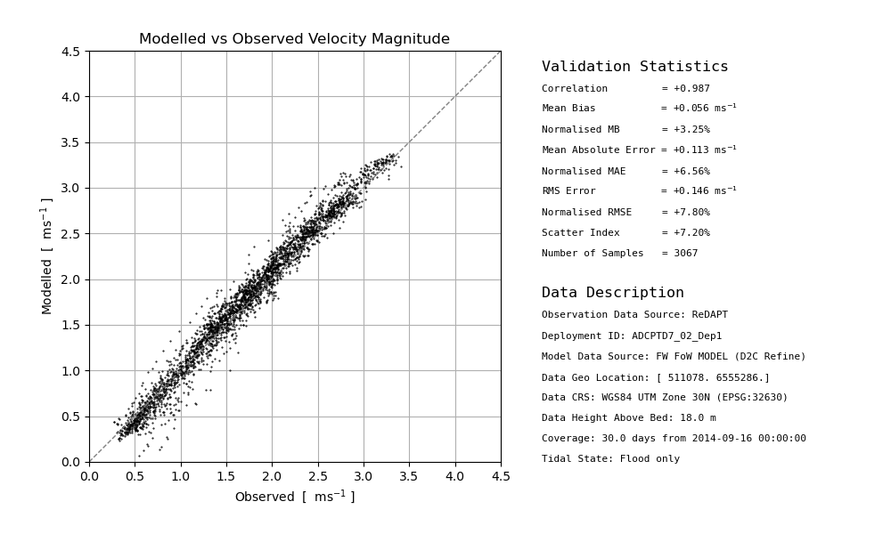
Figure 16. Validation of Falls of Warness D2C model velocity magnitude against the ReDAPT TD7_02 measurement for the DeepGenIV turbine hub height for flood tides.

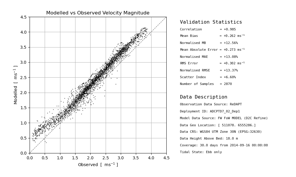
Figure 17. Validation of Falls of Warness D2C model velocity magnitude against the ReDAPT TD7_02 measurement for the DeepGenIV turbine hub height for ebb tides.

The summary graphics for the FoW D2C model velocity directions at the two measurement sites for the DeepGenIV hub height are shown below.

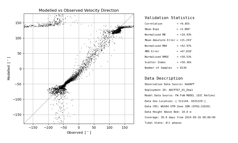
Figure 18. Validation of Falls of Warness D2C model velocity direction against the ReDAPT TD7_01 measurement for the DeepGenIV turbine hub height for the all tide states.

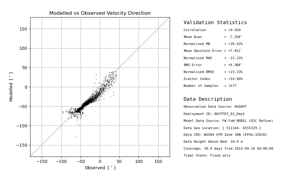
Figure 19. Validation of Falls of Warness D2C model velocity direction against the ReDAPT TD7_01 measurement for the DeepGenIV turbine hub height for flood tides.

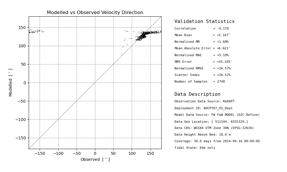
Figure 20. Validation of Falls of Warness D2C model velocity direction against the ReDAPT TD7_01 measurement for the DeepGenIV turbine hub height for ebb tides.

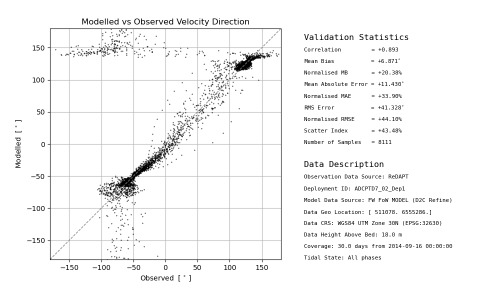
Figure 21. Validation of Falls of Warness D2C model velocity direction against the ReDAPT TD7_02 measurement for the DeepGenIV turbine hub height for the all tide states.

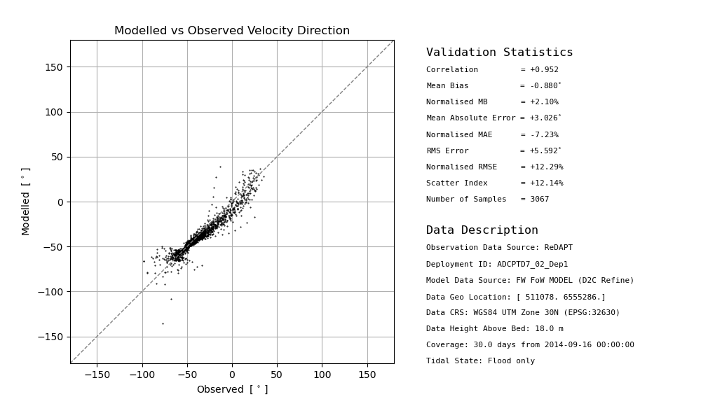
Figure 22. Validation of Falls of Warness D2C model velocity direction against the ReDAPT TD7_02 measurement for the DeepGenIV turbine hub height for flood tides.

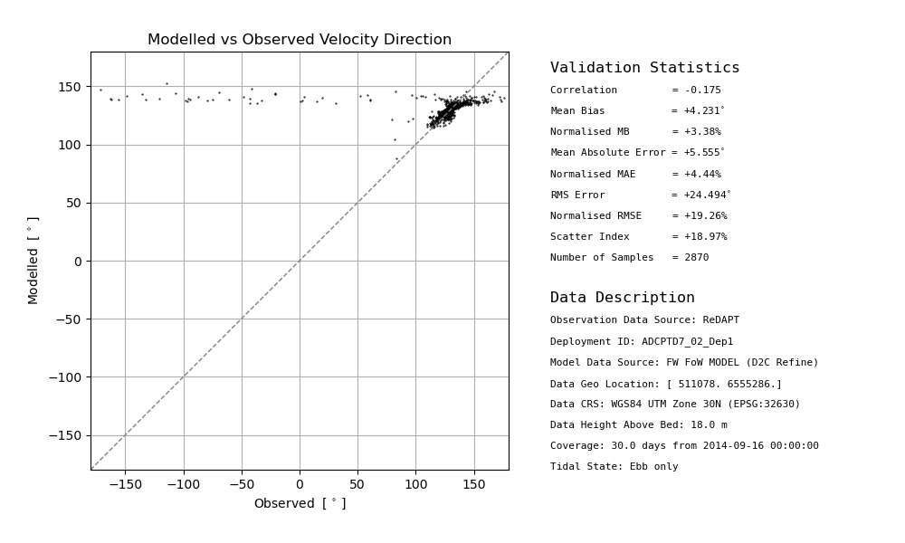
Figure 23. Validation of Falls of Warness D2C model velocity direction against the ReDAPT TD7_02 measurement for the DeepGenIV turbine hub height for ebb tides.

FoW Data Analysis

The above described validataion process was applied to the FASTWATER Base model, FoW D2C model and the FoW VORT model, for the two ReDAPT intstrument locations and for the three difference turbine classes. The quantify the model perfomance and determine whether the models are capture all of key variability, the data generated were tabulated to show the underlying patterns of model behaviour.

The most fundamental test is around the flow characterisation parameters for the peak flood and ebb directions and the flood/ebb asymmetry in direction. The follow two tables summarise these data for the two locations.

Table 5: Flow characterisation direction parameters for the TD7_01 instrument location

Turbine	Sabell D10			Alstrom DeepGenIV			Orbial Marine 02
Data Source	Flood	Ebb	Asymm	Flood	Ebb	Asymm	Flood	Ebb	Asymm
ReDAPT	-41.6	126.9	168.5	-42.8	130.1	172.9	-45.2	134.0	179.2
FW Base Model	-54.0	128.1	178.0	-54.4	128.5	177.1	-55.6	128.8	175.7
FoW D2C Model	-47.8	127.3	175.1	-48.6	128.9	177.5	-50.8	130.9	178.2
FoW VORT Model	-47.4	127.6	175.1	-48.3	129.4	177.6	-50.4	131.3	178.2

At location TD7_01, the in situ ReDAPT data show that the ebb/flood flow directional asymmetry decrease with height above the bed, ranging from 168.5 \(^{\circ}\) at 18m above bed to 179.2 \(^{\circ}\) at 14m below the surface (approimately 31m above bed). The models replicate this pattern but with a smaller directional variation with height above the bed ( Fow VORT Model - 175.1 \(^{\circ}\) to 178.2 \(^{\circ}\)). The low-resolution FW BASE Model is the least effective at reprocucing the veritcal variation in flow directional asymmetry. At this location there is no measurable difference in the D2C and VORT models abilities to replicate the flow directional asymmetry.

Table 6: Flow characterisation direction parameters for the TD7_01 instrument location

Turbine	Sabell D10			Alstrom DeepGenIV			Orbial Marine 02
Data Source	Flood	Ebb	Asymm	Flood	Ebb	Asymm	Flood	Ebb	Asymm
ReDAPT	-48.5	122.8	171.3	-49.5	125.6	175.1	-51.4	129.0	179.6
FW Base Model	-53.8	126.5	179.7	-54.2	127.1	178.7	-55.4	127.6	177.0
FoW D2C Model	-48.0	126.8	174.8	-48.8	128.2	177.0	-50.9	129.8	179.3
FoW VORT Model	-47.4	127.4	174.8	-48.3	129.7	177.0	-50.4	130.1	179.5

At location TD7_02, the in situ ReDAPT data shows the pattern of ebb/flood flow directional asymmetry decrease with height above the bed, but with a reduced range of 171.3 \(^{\circ}\) at 18m above bed to 179.6 \(^{\circ}\) at 14m below the surface (approimately 31m above bed). The models replicate this pattern but with a smaller directional variation with height above the bed ( Fow VORT Model - 174.8 \(^{\circ}\) to 179.5 \(^{\circ}\)). The low-resolution FW BASE Model is the least effective at reprocucing the veritcal variation in flow directional asymmetry. At this location there is the VORT does marginally better at replicating the near-surface flow direction asymetry compared with the D2C model, otherwise these two model produce simlar estiamtes of the flow directional asymmetry.

The detail in the validation statistics is more complex. The data will be present by validation metric. The statistical metrics calculates are: (1) correlation coefficient R, (2) mean bias MB, (2) mean absolute error MAE, (4) root-mean-square error RMSE, and (5) scatter index SI. These are further separated into all tide states (flood+ebb), flood only, and ebb only, for each of the three example turbine hub heights. We will only present the tabulated data for R, MB, and RMSE, as these are sufficient to determine the model behaviour compared to the observations.

Table 7: Flow magintude validation statistics at TD7_01: R

Tide State	All			Flood only			Ebb only
Model	Base	D2C	VORT	Base	D2C	VORT	Base	D2C	VORT
D10 [ 11m AB ]	0.968	0.967	0.947	0.980	0.983	0.971	0.978	0.982	0.982
DGIV [ 18m AB ]	0.928	0.967	0.947	0.981	0.985	0.976	0.979	0.982	0.985
O2 [ 14m BS ]	0.928	0.972	0.960	0.982	0.984	0.978	0.950	0.957	0.984

For all models, the flow magintude data at location TD7_01 are highly correlated (R > 0.92) for all models and depth locations. When separated into flood and ebb tides, in general the flood tide is better represented by the BASE and D2C models, whereas teh ebb tide is better represented by the VORT model. Both the BASE and D2C models give a lower correlation near the surface.

Table 8: Flow magintude validation statistics at TD7_02: R

Tide State	All			Flood only			Ebb only
Model	Base	D2C	VORT	Base	D2C	VORT	Base	D2C	VORT
D10 [ 11m AB ]	0.973	0.972	0.960	0.981	0.984	0.978	0.980	0.982	0.984
DGIV [ 18m AB ]	0.974	0.975	0.966	0.983	0.985	0.982	0.980	0.982	0.985
O2 [ 14m BS ]	0.926	0.977	0.970	0.985	0.986	0.986	0.980	0.983	0.981

For all models, the flow magintude data at location TD7_02 are highly correlated (R > 0.92) for all models and depth locations. When separated into flood and ebb tides, all models correlate to a good level at for both states of the tide.

Table 9: Flow magintude validation statistics at TD7_01: MB (%)

Tide State	All			Flood only			Ebb only
Model	Base	D2C	VORT	Base	D2C	VORT	Base	D2C	VORT
D10 [ 11m AB ]	1.0	8.5	13.5	2.1	1.9	5.0	8.0	17.2	26.2
DGIV [ 18m AB ]	2.2	7.8	13.0	-3.4	1.6	4.7	9.9	16.9	26.5
O2 [ 14m BS ]	8.5	13.6	18.7	-3.3	1.4	4.6	26.7	32.7	44.0

The mean bias is more informative than the correlation; this shows differences in estimtation of the flow speeds. The mean bias has been presented as a percentage (%) bias. There are three key patterns for the data at location TD7_01. The BASE model bias increases with height above bed, whereas the bias in the D2C and VORT models is higher at the lower and upper levels, compared with mid-water. The bias is significantly lower for the flood tide for all model. The bias in the VORT model is higher than that of the D2C model.

Table 10: Flow magintude validation statistics at TD7_02: MB (%)

Tide State	All			Flood only			Ebb only
Model	Base	D2C	VORT	Base	D2C	VORT	Base	D2C	VORT
D10 [ 11m AB ]	1.1	8.7	12.4	-2.7	4.0	6.6	7.2	16.7	23.1
DGIV [ 18m AB ]	-0.7	6.4	10.2	-3.0	3.4	6.0	4.4	12.9	19.2
O2 [ 14m BS ]	-2.5	9.6	8.3	-3.6	2.7	5.6	1.7	9.2	15.2

There patterns for the mean bias data at location TD7_02 are slightly different. The BASE model bias increases with height above bed, whereas the bias in the D2C and VORT models both decrease with height above bed. The bias is significantly lower for the flood tide for all model. The bias in the VORT model is higher than that of the D2C model. Again the bias on the ebb tide is significantly higher for all models compared with the flood tide.

Table 11: Flow magintude validation statistics at TD7_01: RMSE (%)

Tide State	All			Flood only			Ebb only
Model	Base	D2C	VORT	Base	D2C	VORT	Base	D2C	VORT
D10 [ 11m AB ]	12.1	15.1	20.3	8.5	8.0	9.7	11.4	17.5	25.4
DGIV [ 18m AB ]	12.7	14.7	19.8	8.6	7.5	9.0	12.8	17.3	25.6
O2 [ 14m BS ]	20.4	22.7	27.8	8.4	7.8	9.3	27.5	32.3	42.1

The RMSE tells us somthing about the spread of the difference in the model predictions compared with in situ data. At location TD7_01 the percentage RMSE is relatively high and increases with height above the bed. The RMSE on the ebb tide is higher than that on the flood tide. The D2C model has a lower RMSE than the VORT model.

Table 12: Flow magintude validation statistics at TD7_02: RMSE (%)

Tide State	All			Flood only			Ebb only
Model	Base	D2C	VORT	Base	D2C	VORT	Base	D2C	VORT
D10 [ 11m AB ]	11.1	15.0	18.5	8.4	8.7	9.8	10.1	17.3	22.7
DGIV [ 18m AB ]	10.5	12.9	16.1	8.2	8.2	9.0	8.8	13.9	19.0
O2 [ 14m BS ]	10.6	11.2	13.9	8.0	8.4	8.4	8.3	14.1	15.7

At location TD7_02 the percentage RMSE is also relatively, but tends to decrease with height above the bed. The RMSE on the ebb tide is higher than that on the flood tide. The D2C model again has a lower RMSE than the VORT model.

Interpretation of the validation statistics

Implication:

1. Bottom boundary layer poorly resolved (more vertical layers near bed)

2. Bottom friction too low (increased drag will modify bottom boundary Ekman layer formation)

3. Bottom topography not fully resolved (low-resoltiom bathymetry may have smoothed out local structures that will cause the flow to veer near the bed).

4. Vertical velocity diffusion rates to low - related to replication of vertical structure with number of layers used.

SIMEC-Atlantis MeyGen Site - Inner Sound, Pentland Firth

PF_IS Model Design Specification

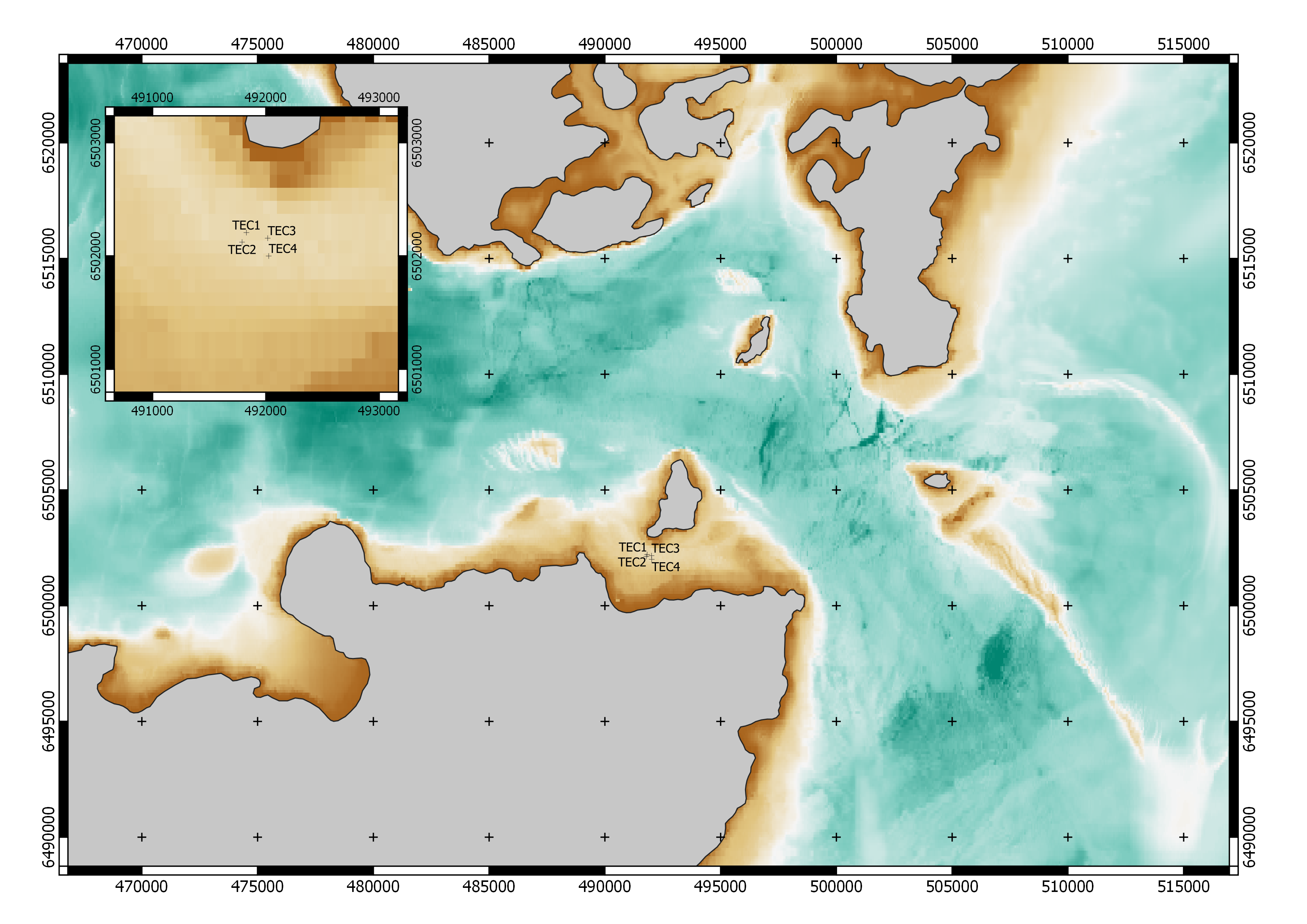
Figure 24. Inner Sound site map. The locations of the four operation MeyGen tidal turbines. The inset shows the proximity of turbines to Stroma.

PF_IS Mesh Construction

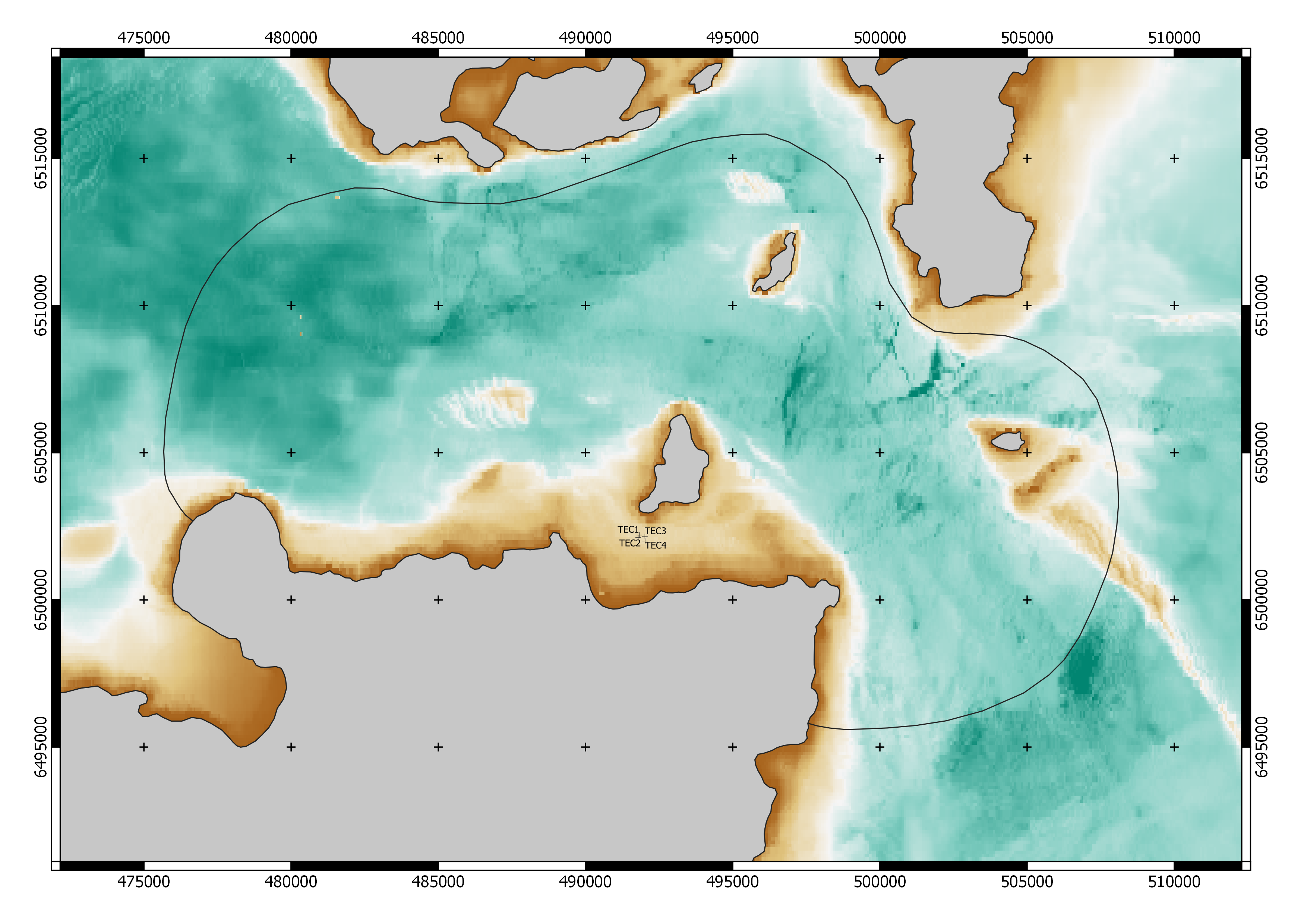
Figure 25. Inner Sound refinement region used to build the distance-to-coast sub-mesh. The extent of the area aims to capture all of the large-scale dynamics assoicted with the flow through Pentland Firth and island wakes formed off Stroma and Swona.

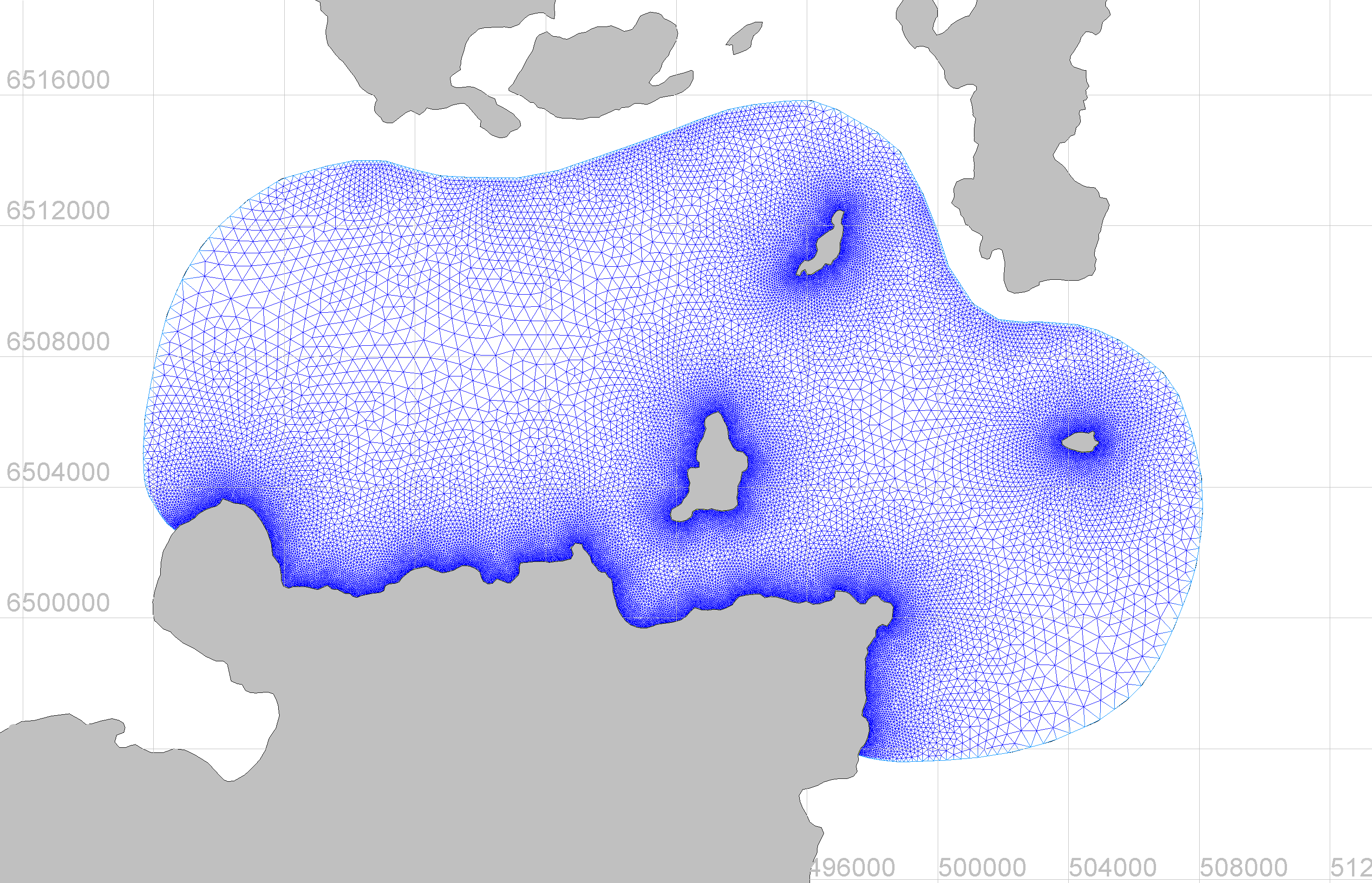
Figure 26. Inner Sound refinement sub-mesh generated in BlueKenue using the distance-to-coast density data.

The full mesh was generated around the sub-mesh using the 250m resolution coastline data with a growth rate of 1.2 and a maximum outer domain target edge length of 10km. The resulting key mesh parameters fro the sub-mesh and full mesh are summarised in the table below.

Table: Inner Sound model mesh characterisation parameters

Mesh Parameter	Sub-Mesh	Full Mesh
Number of Nodes	31553	72644
Number of Edge Nodes	2299	10048
Minimum Edge Length	14.1m	14.1m
Maximum Edge Length	699.2m	14022.2m
Mean Edge Length	97.7m	324.2m

The boundary conditions for this model are the same as those used in Case Study 1 above.

PF_IS Numerical Scheme

The model is run in 3D mode using the non-hydrostatic setting.

Coriolis forcing is turned on, with the coefficient set to \(1.25 \times 10^{-4}\) (this corresponds approximately to the value at the Falls of Warness).

Tidal boundary forcing is via the tidal harmonics provided by the OSU TOPEX European Shelf (2008) tidal atlas data. The minor constituent interference is included in the computation of the tidal forcing.

Liquid boundary conditions solved using the Thompson method based on characteristics.

Wetting/Drying is turned on with the N-S equations solved everywhere with a free-surface gradient correction on tidal flats. Negative depths a corrected using a flux control method. To optimise computation time, void volumes are skipped.

Horizontal turbulence is modelled using the Smagorinsky scheme (recommended in the OpenTelemac Users Guide).

Vertical turbulence is modelled using a Prandtl mixing length parematerisation, with a coefficient for the vertical diffusion of velocity set to \(1.0 \times 10^{-6}\), and the Munk and Anderson damping function applied. The turbulence regime for the solid boundaries is set to rough.

Preconditioning for the propagation steps and Poisson Pressure Equation are set to diagnonal and direct solver on the vertical respectively.

PF_IS Data Analysis

The process_pfis.py script in the /scripts/modelValidation directory was used to post process the timeseries of data extracted from the refined model at the locations of the TEC1 and TEC2 tidal turbines. This processing includes the flow characterisation and extraction of the power-weigthed rotor-averaged (PWRA) velocity in the along-stream direction (taken to be the peak ebb and flood directions defined by the flow characterisation).

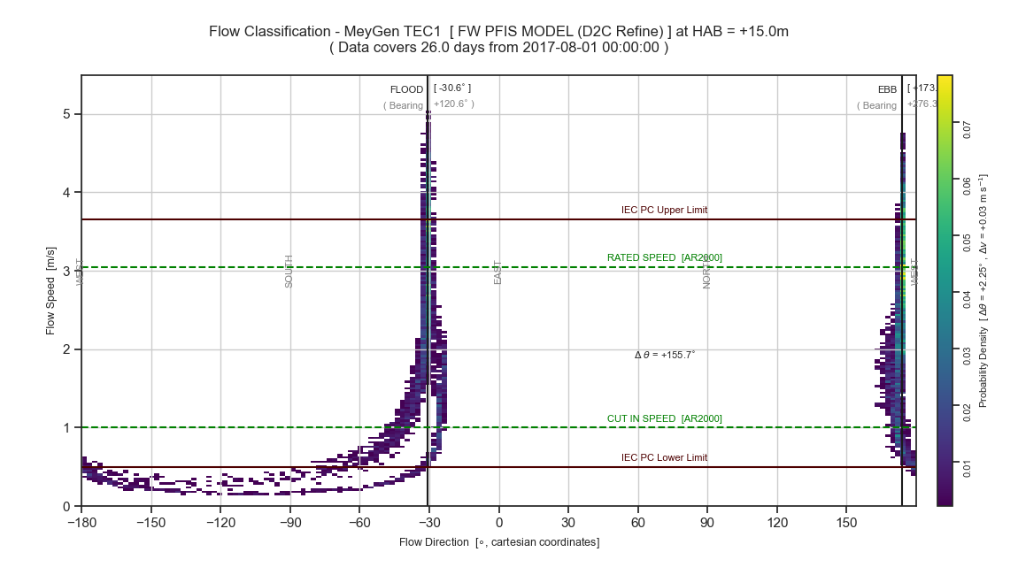
Figure 27. Inner Sound flow characterisation for TEC1.

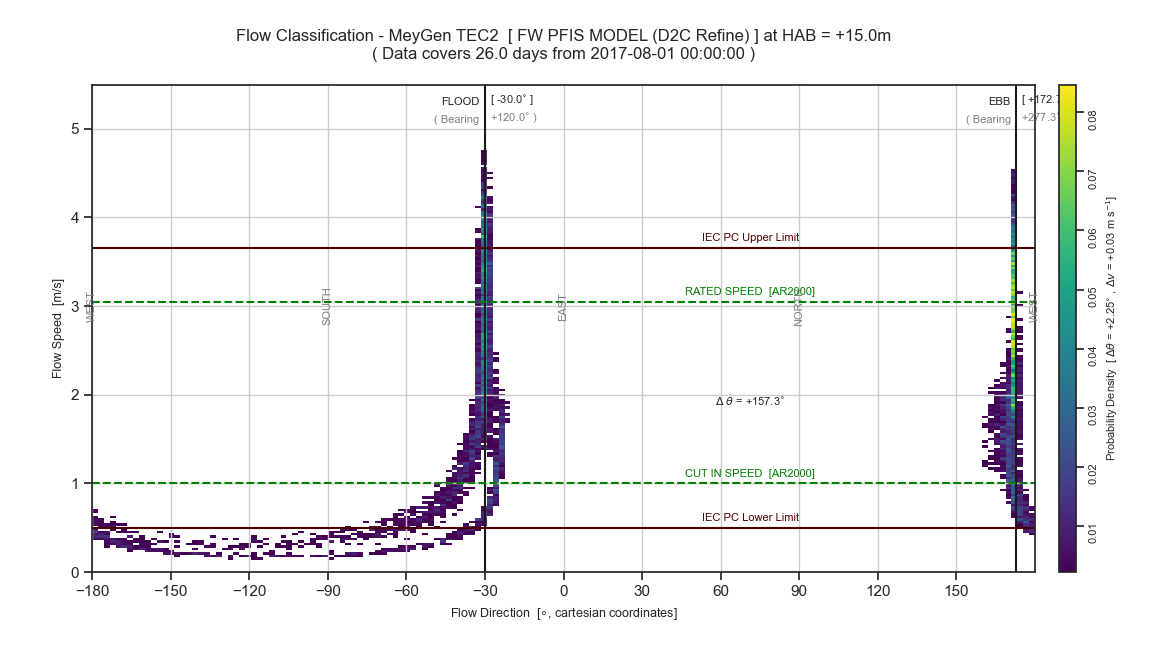
Figure 28. Inner Sound flow characterisation for TEC2.

The flow characterisation diagrams for the two TEC locations TEC1 and TEC2 are shown in Figure 27 and Figure 28 respectively. At both sites the peak flood speed is sligthly higher than the ebb, but the peak flow speeds at TEC2 are lower than those at TEC1. Both site exhibit a strong asymmetry in the flood/ebb directions. i.e. the flow is far from rectilinear (\(\Delta\theta = 180\circ\)). This asymmetry is driven by flow curvature around the headland of the southern end of Stroma.

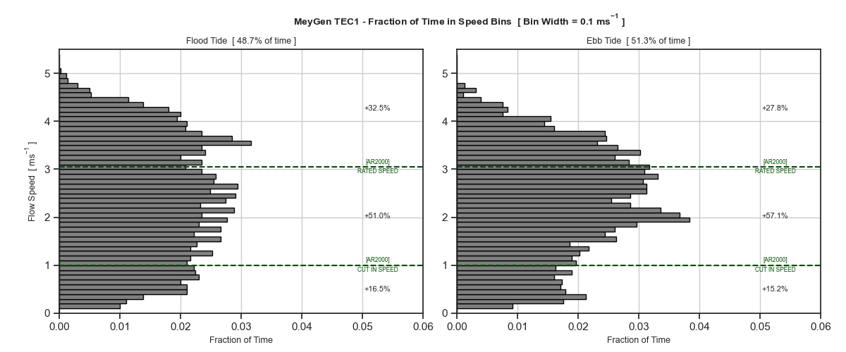
Figure 29. Inner Sound distribution of flow speeds for TEC1.

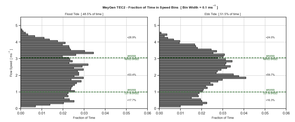
Figure 30. Inner Sound distribution of flow speeds for TEC2.

Figure 29 and Figure 30 show histograms of the flow speeds separated into flood and ebb phases for TEC1 and TEC2 respectively. The turbine cut-in and rated speeds are included with the percentage of time spent with the three main speed ranges. On average TEC1 spends more in in flows above the cut-in speed and above the rated speed than TEC2. Based on this observation, the expectation is that TEC1 will generate more power than TEC2.

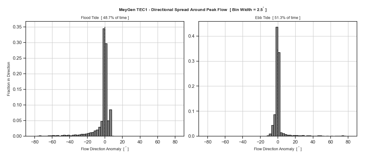
Figure 31. Inner Sound distribution of flow directions for TEC1.

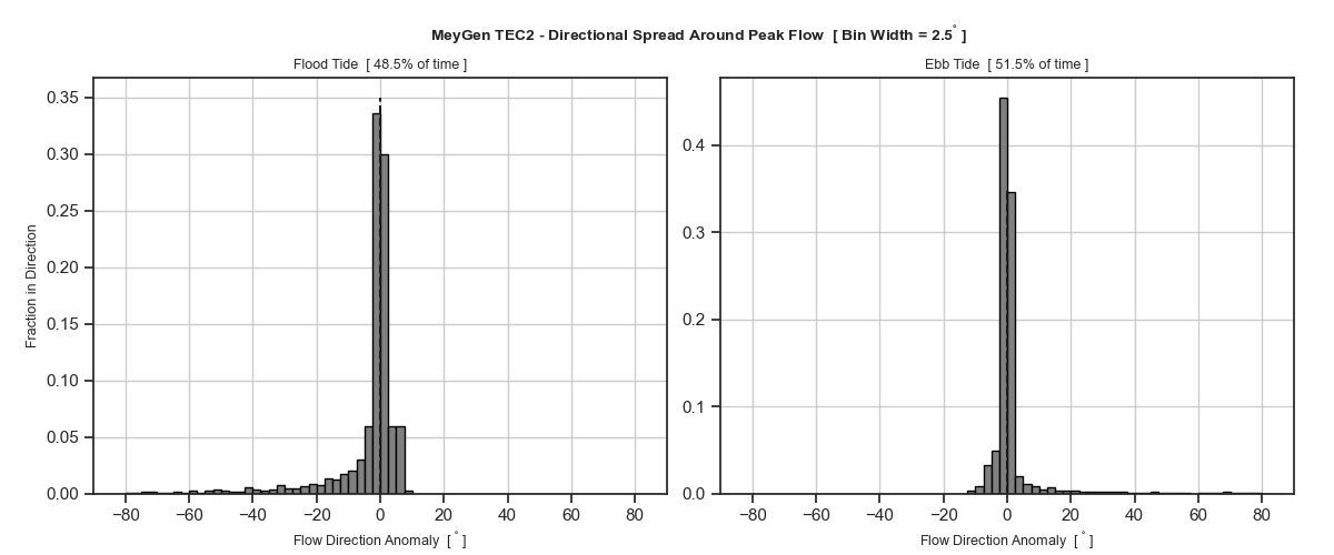
Figure 32. Inner Sound distribution of flow directions for TEC2.

Figure 31 and Figure 32 show histograms of the flow direction about the peak flow direction separated into flood and ebb phases for TEC1 and TEC2 respectively. Both site show minimal variation about the peak directions for both tides, indicating that these locations are not stongly affected by large-scale coherent eddy structures.

The tidal energy converters install at TEC1 and TEC2 locations are Atlantis AR1500 turbines. These have a 18m rotor diameter, and the hub is approximately 15m above the seabed. Functions for extracing the The PWRA velocity data from a timeseries of velocity profiles is included in the :py:mod:`fastwater.analysis.flowChar.py`_ module. The timeseries of PWRA along-stream velocity data was converted into an estimate of the power production using the standard simplified equation:

\(P = 0.5 \rho_{sw} A_{rot} U_{PWRA}^{3} C_{p}\)

where \(\rho_{sw}\) is the density of seawater, \(A_{rot}\) is the turbines rotor swept area, \(U_{PWRA}\) is the power-weighted rotor-averaged in-flow velocity, and \(C_{p}\) is the power coefficient for the turbine. More correctly, a power curve should be used to estimate the power production, as this is depdendent on the flow speed, but for the purposes of the this analysis the simplified approximation is sufficient. Figure 33 shows the two power timeseries over-plotted, indicating that more power is generated at the location of TEC1 compared with the TEC2 location.

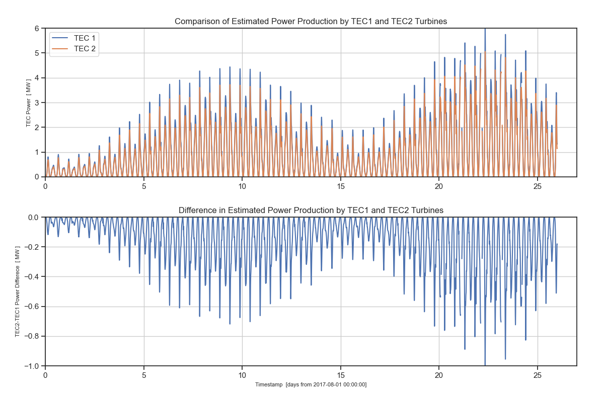
Figure 33. Inner Sound estimated power production over model run period. The upper panel shows the over-plotted power estimates for the two turbine locations, TEC1 and TEC2, and the lower panel shows the difference in the estimated power production.

By integrating the power over time the total energy production can be estimated for both locations, this shows that the energy yield at the TEC2 is 86.1% of that at the TEC1 location, i.e. the TEC2 energy yield is 13.9% lower based on this models predictions. If the yield is calculated for only in-flow speeds greater than the turbine cut-in speed, then relative TEC2 yield difference only marginally higher - in this case the TEC2 energy yield is 14.0% lower.

Validation against in situ measurements would help determine whether this model needs further calibration to the vertical profile shape. If the shape is over estimating the near-bed flows, then the PWRA velocities will be over-estimated.

Developers often used 2-D shallow-water tidal models to do their site assessment. To replicate the possible impact of using a 2-D simulation the power was calculated using the depth-averaged velocity data. This is not strcitly the same as the results from a 2-D solution to the shallow-water euqations as these do not have the ability to represent the 3-D recirculation patterns, but the depth-average velocity will be representative.

Using the depth aveaged velocity to calculate the turbine power and total energy production over the simulation period estiamted that the energy at TEC2 is 89.4% of that at TEC1. This suggests that using a 2-D simulation will probably lead to an over estimation of the energy produciton, but still indicates that the production at TEC2 is lower than at TEC1.